Precipitation Variability and Extreme Events

Precipitation Variability and Extreme Events#

Content creators: Will Gregory, Laura Paccini, Raphael Rocha

Content reviewers: Paul Heubel, Jenna Pearson

Content editors: Paul Heubel

Production editors: Paul Heubel, Konstantine Tsafatinos

Our 2024 Sponsors: CMIP, NFDI4Earth

Project Background#

In this project, you will explore rain gauge and satellite data from the CHIRPS data set to extract rain estimates and land surface reflectance, respectively. These data will enable identification of extreme events in your region of interest. Besides investigating the relationships between these variables, you are encouraged to study the impact of extreme events on changes in vegetation.

Project Template#

Data Exploration Notebook#

Project Setup#

# google colab installs

#!pip install --quiet s3fs boto3 botocore

# Imports

import numpy as np
import matplotlib.pyplot as plt
import xarray as xr
import pooch
import os
import tempfile
import pandas as pd
import s3fs
import boto3
import botocore
import datetime

Helper functions#

Figure settings#

CHIRPS Version 2.0 Global Daily 0.25°#

The Climate Hazards Group InfraRed Precipitation with Station data (CHIRPS) is a high-resolution precipitation dataset developed by the Climate Hazards Group at the University of California, Santa Barbara. It combines satellite-derived precipitation estimates with ground-based station data to provide gridded precipitation data at a quasi-global scale between 50°S-50°N.

Indices for Extreme Events#

The Expert Team on Climate Change Detection and Indices (ETCCDI) has defined various indices that focus on different aspects such as duration or intensity of extreme events. The following functions provide examples of how to compute indices for each category. You can modify these functions to suit your specific needs or create your own custom functions. Here are some tips you can use:

Most of the indices require daily data, so in order to select a specific season you can just use xarray to subset the data. Example:

daily_precip_DJF = data_chirps.sel(time=data_chirps['time.season']=='DJF')

A common threshold for a wet event is precipitation greater than or equal to \(1 \text{ mm}/\text{day}\), while a dry (or non-precipitating) event is defined as precipitation less than \(1 \text{ mm}/\text{day}\).
Some of the indices are based on percentiles. You can define a base period climatology to calculate percentile thresholds, such as the 5th, 10th, 90th, and 95th percentiles, to determine extreme events (cf. in particular W2D3).

def calculate_cdd_index(data):
    """
    This function takes a daily precipitation dataset as input and calculates
    the Consecutive Dry Days (CDD) index, which represents the longest sequence
    of consecutive days with precipitation less than 1mm. The input data should
    be a DataArray with time coordinates, and the function returns a DataArray
    with the CDD values for each unique year in the input data.
    Parameters:
    ----------
      - data (xarray.DataArray): The input daily precipitation data should be
      a dataset (eg. for chirps_data the DataArray would be chirps_data.precip)
    Returns:
    -------
      - cdd (xarray.DataArray): The calculated CDD index

    """
    # create a boolean array for dry days (PR < 1mm)
    dry_days = data < 1
    # initialize CDD array
    cdd = np.zeros(len(data.groupby("time.year")))
    # get unique years as a list
    unique_years = list(data.groupby("time.year").groups.keys())
    # iterate for each day
    for i, year in enumerate(unique_years):
        consecutive_trues = []
        current_count = 0
        for day in dry_days.sel(time=data["time.year"] == year).values:
            if day:
                current_count += 1
            else:
                if current_count > 0:
                    consecutive_trues.append(current_count)
                    current_count = 0
        if current_count > 0:
            consecutive_trues.append(current_count)
        # print(consecutive_trues)
        # CDD is the largest number of consecutive days
        cdd[i] = np.max(consecutive_trues)
    # transform to dataset
    cdd_da = xr.DataArray(cdd, coords={"year": unique_years}, dims="year")
    return cdd_da

# code to retrieve and load the data

years = range(1981,2024) # the years you want. we want 1981 till 2023
file_paths = ['https://data.chc.ucsb.edu/products/CHIRPS-2.0/global_daily/netcdf/p25/chirps-v2.0.' + str(year) + '.days_p25.nc' for year in years] # the format of the files
filenames = ['chirps-v2.0.'+str(year)+'.days_p25.nc' for year in years] # the format of the files

downloaded_files=[ pooch_load(fpath,fname) for (fpath,fname) in zip(file_paths,filenames)] # download all of the files

#### open data via xarray
chirps_data = xr.open_mfdataset(
    downloaded_files, combine="by_coords"
)  # open the files as one dataset

We can now visualize the content of the dataset.

# code to print the shape, array names, etc of the dataset
chirps_data

<xarray.Dataset> Size: 36GB
Dimensions:    (latitude: 400, longitude: 1440, time: 15705)
Coordinates:
  * latitude   (latitude) float32 2kB -49.88 -49.62 -49.38 ... 49.38 49.62 49.88
  * longitude  (longitude) float32 6kB -179.9 -179.6 -179.4 ... 179.6 179.9
  * time       (time) datetime64[ns] 126kB 1981-01-01 1981-01-02 ... 2023-12-31
Data variables:
    precip     (time, latitude, longitude) float32 36GB dask.array<chunksize=(61, 67, 240), meta=np.ndarray>
Attributes: (12/15)
    Conventions:       CF-1.6
    title:             CHIRPS Version 2.0
    history:           created by Climate Hazards Group
    version:           Version 2.0
    date_created:      2015-10-07
    creator_name:      Pete Peterson
    ...                ...
    reference:         Funk, C.C., Peterson, P.J., Landsfeld, M.F., Pedreros,...
    comments:           time variable denotes the first day of the given day.
    acknowledgements:  The Climate Hazards Group InfraRed Precipitation with ...
    ftp_url:           ftp://chg-ftpout.geog.ucsb.edu/pub/org/chg/products/CH...
    website:           http://chg.geog.ucsb.edu/data/chirps/index.html
    faq:               http://chg-wiki.geog.ucsb.edu/wiki/CHIRPS_FAQ

NOAA Fundamental Climate Data Records (FCDR) AVHRR Land Bundle - Normalized Difference Vegetation Index#

As we learned in the W1D3 tutorials, all the National Atmospheric and Oceanic Administration Climate Data Record (NOAA-CDR) datasets are available both at NOAA National Centers for Environmental Information (NCEI) and commercial cloud platforms. See the link here. We are accessing the data directly via the Amazon Web Service (AWS) cloud storage space.

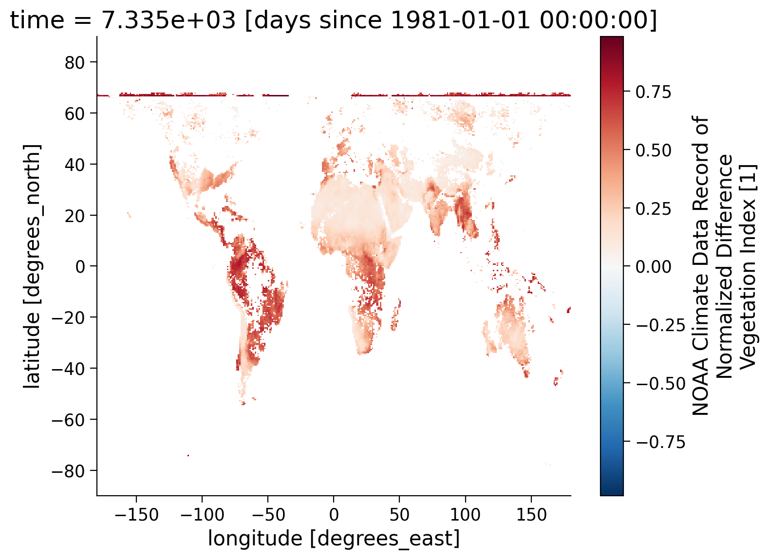
For this project, we recommend using the Normalized Difference Vegetation Index (NDVI). It is one of the most commonly used remotely sensed indices. It measures the “greenness” of vegetation and is useful in understanding vegetation density and assessing changes in plant health. For example, NDVI can be used to study the impacts of droughts, heatwaves, and insect infestations on plants covering Earth’s surface. A good overview of this index from this particular sensor can be accessed here.

Recall what we learned in W1D3 Tutorial 3, the data files on AWS are named systematically:

Sensor name: AVHRR
Product category: Land
Product version: v005
Product code: AVH13C1
Satellite platform: NOAA-07
Date of the data: 19810624
Processing time: c20170610041337 (This will change for each file based on when the file was processed)
File format: .nc (netCDF-4 format)

In other words, if we are looking for the data of a specific day, we can easily locate where the file might be.

For example, if we want to find the AVHRR data for the day of 2002-03-12 (or March 12, 2002), you can use:

s3://noaa-cdr-ndvi-pds/data/2002/AVHRR-Land_v005_AVH13C1_*_20020312_c*.nc

The reason that we put * in the above directory is that we are not sure about what satellite platform this data is from and when the data was processed. The * is called a wildcard, and is used because we want all the files that contain our specific criteria, but do not want to have to specify all the other pieces of the filename we are not sure about yet. It should return all the data satisfying that initial criteria and you can refine further once you see what is available. Essentially, this first step helps to narrow down the data search. You can then use this to create datasets from the timeframe of your choosing.

Note the download might take up to hours depending on your time frame of interest and your device. Choose your time frame wisely before taking action to avoid unnecessary data retrieval amounts.

# we can access the data similar to Tutorial 3 of W1D3
# to access the NDVI data from AWS S3 bucket, we first need to connect to s3 bucket

fs = s3fs.S3FileSystem(anon=True)
client = boto3.client('s3', config=botocore.client.Config(signature_version=botocore.UNSIGNED)) # initialize aws s3 bucket client
# choose a date of interest, we pick its year or month while defining the file_location
date_sel = datetime.datetime(2001,1,1,0)

file_location = fs.glob('s3://noaa-cdr-ndvi-pds/data/'
                        + date_sel.strftime('%Y')
                        + '/AVHRR-Land_v005_AVH13C1_*'
                        + date_sel.strftime("%Y%m") # or "%Y" for the entire year
                        + '*_c*.nc') # the files we want for a whole year/month
files_for_pooch=[pooch_load('http://s3.amazonaws.com/'+file,file) for file in file_location]

ds = xr.open_mfdataset(files_for_pooch, combine="by_coords", decode_times=False)  # open the file
ds

<xarray.Dataset> Size: 11GB
Dimensions:    (latitude: 3600, longitude: 7200, time: 31, ncrs: 1, nv: 2)
Coordinates:
  * latitude   (latitude) float32 14kB 89.97 89.93 89.88 ... -89.93 -89.97
  * longitude  (longitude) float32 29kB -180.0 -179.9 -179.9 ... 179.9 180.0
  * time       (time) float32 124B 7.305e+03 7.306e+03 ... 7.334e+03 7.335e+03
Dimensions without coordinates: ncrs, nv
Data variables:
    crs        (time, ncrs) int16 62B dask.array<chunksize=(1, 1), meta=np.ndarray>
    lat_bnds   (time, latitude, nv) float32 893kB dask.array<chunksize=(1, 3600, 2), meta=np.ndarray>
    lon_bnds   (time, longitude, nv) float32 2MB dask.array<chunksize=(1, 7200, 2), meta=np.ndarray>
    NDVI       (time, latitude, longitude) float32 3GB dask.array<chunksize=(1, 1200, 2400), meta=np.ndarray>
    TIMEOFDAY  (time, latitude, longitude) float64 6GB dask.array<chunksize=(1, 1200, 2400), meta=np.ndarray>
    QA         (time, latitude, longitude) int16 2GB dask.array<chunksize=(1, 3600, 7200), meta=np.ndarray>
Attributes: (12/48)
    title:                                  Normalized Difference Vegetation ...
    institution:                            NASA/GSFC/SED/ESD/HBSL/TIS/MODIS-...
    Conventions:                            CF-1.6, ACDD-1.3
    standard_name_vocabulary:               CF Standard Name Table (v25, 05 J...
    naming_authority:                       gov.noaa.ncei
    license:                                See the Use Agreement for this CD...
    ...                                     ...
    PercentValidDaytimeData:                33.79
    PercentValidDaytimeLand:                33.79
    PercentValidClearDaytimeLand:           4.54
    PercentValidDaytimeLandInCloudShadow:   0.85
    PercentValidClearDaytimeWater:          0.00
    PercentValidDaytimeWaterInCloudShadow:  0.00

If the above downloading procedure is not working as expected, please retrieve the following sample to execute the remaining cells of the notebook. Ask for the help of your project TA to download your data of interest.

# uncomment to get a subsample of AVHRR-Land_v005_AVH13C1_NOAA-16 NDVI data if data retrieval above is not working properly

#fname_ndvi_200101 = 'AVHRR-Land_v005_AVH13C1_NOAA-16_200101.nc'
#link_id_ndvi = "a9v7h"
#url_ndvi_200101 = f"https://osf.io/download/{link_id_ndvi}/"
#
#ds = xr.open_dataset(pooch_load(url_ndvi_200101, fname_ndvi_200101))
#ds

Note that the downloaded satellite data is quality-controlled and flagged accordingly. Please refer to W1D3 Tutorial 3 and others to decipher it. Choose the feasible helper functions, e.g. get_quality_info_AVHRR(QA) depending on the sensor of interest. VIIRS is a state-of-the-art sensor that produces measurements that have been available since 2014. We provide an example of usage in the following.

# AVHRR: function to extract high-quality NDVI data
def get_quality_info_AVHRR(QA):
    """
    QA: the QA value read in from the NDVI data

    High-quality NDVI should meet the following criteria:
    Bit 7: 1 (All AVHRR channels have valid values)
    Bit 2: 0 (The pixel is not covered by cloud shadow)
    Bit 1: 0 (The pixel is not covered by cloud)
    Bit 0:

    Output:
    True: high quality
    False: low quality
    """
    # unpack quality assurance flag for cloud (byte: 1)
    cld_flag = (QA % (2**2)) // 2
    # unpack quality assurance flag for cloud shadow (byte: 2)
    cld_shadow = (QA % (2**3)) // 2**2
    # unpack quality assurance flag for AVHRR values (byte: 7)
    value_valid = (QA % (2**8)) // 2**7

    mask = (cld_flag == 0) & (cld_shadow == 0) & (value_valid == 1)

    return mask

# get the quality assurance value from NDVI data
QA = ds.QA

# create the high quality information mask
mask = get_quality_info_AVHRR(QA)

# check the quality flag mask information
#mask

# mask ndvi data
ndvi_masked = ds.NDVI.where(mask)
ndvi_masked

<xarray.DataArray 'NDVI' (time: 31, latitude: 3600, longitude: 7200)> Size: 3GB
dask.array<where, shape=(31, 3600, 7200), dtype=float32, chunksize=(1, 1200, 2400), chunktype=numpy.ndarray>
Coordinates:
  * latitude   (latitude) float32 14kB 89.97 89.93 89.88 ... -89.93 -89.97
  * longitude  (longitude) float32 29kB -180.0 -179.9 -179.9 ... 179.9 180.0
  * time       (time) float32 124B 7.305e+03 7.306e+03 ... 7.334e+03 7.335e+03
Attributes:
    long_name:      NOAA Climate Data Record of Normalized Difference Vegetat...
    units:          1
    valid_range:    [-1000 10000]
    grid_mapping:   crs
    standard_name:  normalized_difference_vegetation_index

# draw data to an example plot
ndvi_masked.isel(time=30).coarsen(latitude=10).mean().coarsen(longitude=20).mean().plot()

<matplotlib.collections.QuadMesh at 0x7f144849f370>

../../_images/c7e44b650dfe018661e5f656604fb9d6b872169753f6d9949fb0163496bb0d94.png

FAO Data: Cereal Production#

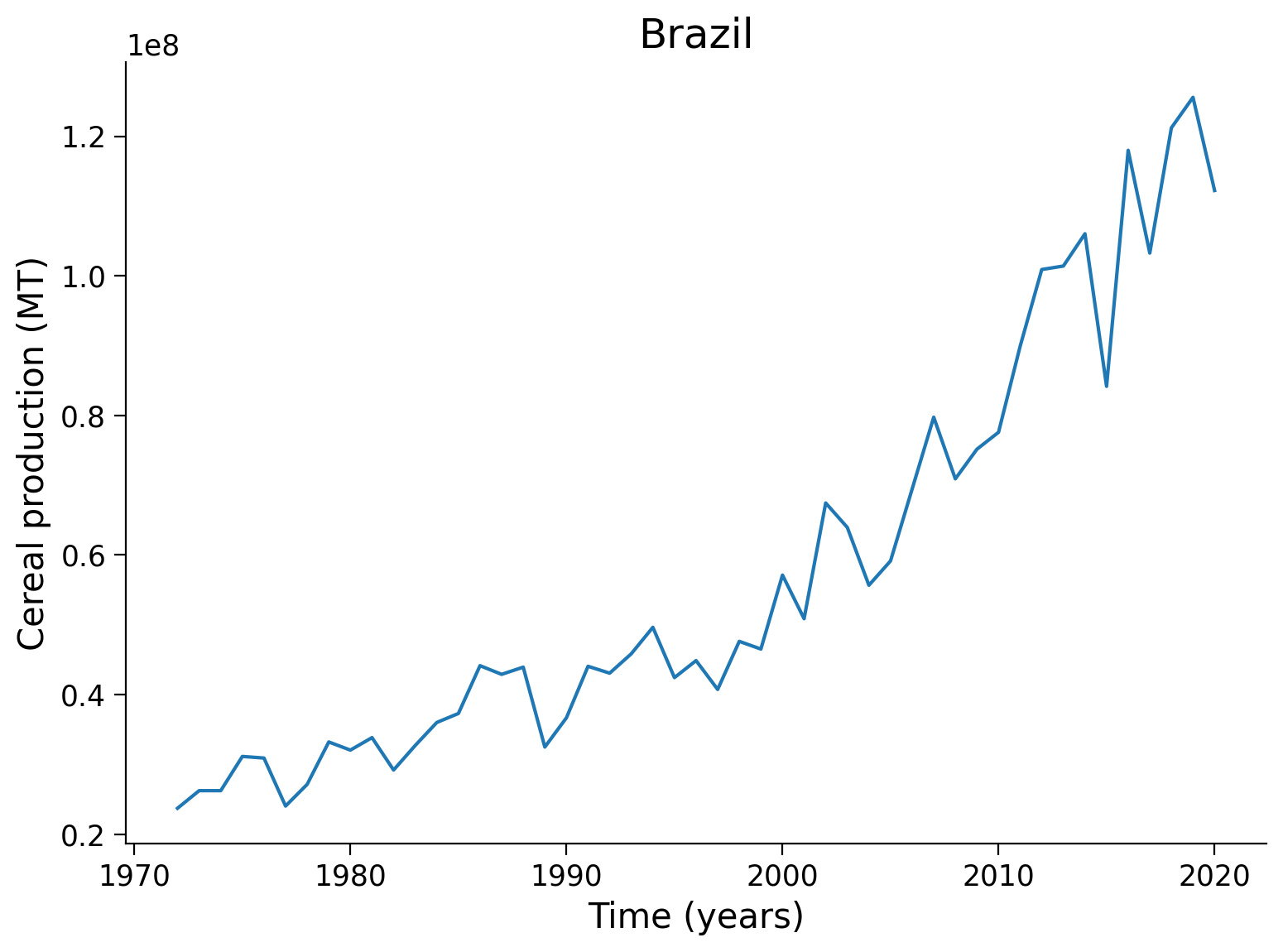
Cereal production is a crucial component of global agriculture and food security. The Food and Agriculture Organization collects and provides data on cereal production, which includes crops such as wheat, rice, maize, barley, oats, rye, sorghum, millet, and mixed grains. The data covers various indicators such as production quantity, area harvested, yield, and production value.

The FAO also collects data on “area harvested”, which refers to the area of land that is being used to grow cereal crops. This information can be valuable for assessing the productivity and efficiency of cereal production systems in different regions, as well as identifying potential areas for improvement. Overall, the FAO’s data on cereal production and land under cereals production is an important resource for policymakers, researchers, and other stakeholders who are interested in understanding global trends in agriculture and food security.

filename_cereal = 'data_cereal_land.csv'

url_cereal = 'https://raw.githubusercontent.com/Sshamekh/Heatwave/f85f43997e3d6ae61e5d729bf77cfcc188fbf2fd/data_cereal_land.csv'

path_cereal = 'shared/data/'
if os.path.exists(path_cereal + filename_cereal):
    ds_cereal_land = pd.read_csv(path_cereal + filename_cereal)
else:
    ds_cereal_land = pd.read_csv(pooch_load(url_cereal,filename_cereal))

ds_cereal_land.head()

	Country Name	Country Code	Series Name	Series Code	1972 [YR1972]	1973 [YR1973]	1974 [YR1974]	1975 [YR1975]	1976 [YR1976]	1977 [YR1977]	...	2012 [YR2012]	2013 [YR2013]	2014 [YR2014]	2015 [YR2015]	2016 [YR2016]	2017 [YR2017]	2018 [YR2018]	2019 [YR2019]	2020 [YR2020]	2021 [YR2021]
0	Afghanistan	AFG	Cereal production (metric tons)	AG.PRD.CREL.MT	3950000	4270000	4351000	4481000	4624000	4147000	...	6379000	6520329	6748023.28	5808288	5532695.42	4892953.97	4133051.85	5583461	6025977	4663880.79
1	Afghanistan	AFG	Land under cereal production (hectares)	AG.LND.CREL.HA	3923100	3337000	3342000	3404000	3394000	3388000	...	3143000	3182922	3344733	2724070	2793694	2419213	1911652	2641911	3043589	2164537
2	Albania	ALB	Cereal production (metric tons)	AG.PRD.CREL.MT	585830	625498	646200	666500	857000	910400	...	697400	702870	700370	695000	698430	701734	678196	666065	684023	691126.7
3	Albania	ALB	Land under cereal production (hectares)	AG.LND.CREL.HA	331220	339400	334040	328500	350500	357000	...	142800	142000	143149	142600	148084	145799	140110	132203	131310	134337
4	Algeria	DZA	Cereal production (metric tons)	AG.PRD.CREL.MT	2362625	1595994	1480275	2680452	2313186	1142509	...	5137455	4912551	3435535	3761229.6	3445227.37	3478175.14	6066252.82	5633596.78	4393336.75	2784017.29

5 rows × 54 columns

# example
country = 'Brazil'
unit = 'MT' # metric tons

ds_cereal_land_brazil = ds_cereal_land[
(ds_cereal_land["Country Name"] == country) & (ds_cereal_land["Series Code"] == f'AG.PRD.CREL.{unit}')
].drop(
    ['Country Name', 'Country Code', 'Series Name', 'Series Code'], axis=1
).reset_index( drop=True ).transpose()

ds_cereal_land_brazil.head()

	0
1972 [YR1972]	22703928
1973 [YR1973]	23721606
1974 [YR1974]	26240014
1975 [YR1975]	26238419
1976 [YR1976]	31143200

We can now visualize the content of the dataset.

# example
plt.plot(np.arange(1972,2021,1),ds_cereal_land_brazil[1:].astype(float).values)

# aesthetics
plt.title(f'{country}')
plt.xlabel(f'Time (years)')
plt.ylabel(f'Cereal production ({unit})')

Text(0, 0.5, 'Cereal production (MT)')

../../_images/ee35068742affa42741a6ea04750aa0972de569f0a6f7f7c3bbcda0b28655bfb.png

Now you are all set to address the questions you are interested in!

Q1#

Plot the annual mean of precipitation for three example years (e.g., 2001, 2005, 2016) using the CHIRPS data sets.

Hint: Check out the tutorials from W1D1 (e.g. T4), W1D2 (e.g. T2) and W1D3 (e.g. T5) to recall averaging with xarray.

Q2#

Plot the global mean of land precipitation as a function of time for the last 40 years.

Hint: Check out the tutorials that contain time series calculations e.g. from W1D2 (e.g. T1), W1D3 (e.g. T5) and W1D5 (e.g. T8).

Compute seasonal means for June-August (JJA) and December-February (DJF).

Hint: Check out the code snippet in the Indices for Extreme Events section of this notebook. Furthermore, recall Tutorial 5 of W1D1.

Q3#

Repeat the analysis in Q2 for a selected region of interest. How does this compare with the respective mean precipitation in the northern and southern hemispheres? How does this compare to the global mean?

Hint: Check out tutorials that showed how to select certain regions of interest, e.g. T8 and T9 of W1D1, T1 of W1D2 and others.

Q4#

Examine the time series in your region of interest and identify extreme values.

Hint: Select a method from a predefined list of indices (provided above in Section Indices for Extreme Events) based on relative or absolute thresholds.

Do extreme events occur more often in wet or dry seasons?

Hint: We briefly discussed wet and dry season differences in Tutorial 4 of W1D3 already, however for another data set of monthly frequency namely the Global Precipitation Climatology Project (GPCP) Monthly Precipitation Climate Data Record (CDR) (cf. Tutorial 4 of W1D3). You also examined extreme events on W2D3.