Tutorial 3: Quantifying Uncertainty in Projections

Tutorial 3: Quantifying Uncertainty in Projections#

Week 2, Day 1, An Ensemble of Futures

Content creators: Brodie Pearson, Julius Busecke, Tom Nicholas, Sam Ditkovsky

Content reviewers: Mujeeb Abdulfatai, Nkongho Ayuketang Arreyndip, Jeffrey N. A. Aryee, Younkap Nina Duplex, Sloane Garelick, Paul Heubel, Zahra Khodakaramimaghsoud, Peter Ohue, Jenna Pearson, Abel Shibu, Derick Temfack, Peizhen Yang, Cheng Zhang, Chi Zhang, Ohad Zivan

Content editors: Paul Heubel, Jenna Pearson, Ohad Zivan, Chi Zhang

Production editors: Wesley Banfield, Paul Heubel, Jenna Pearson, Konstantine Tsafatinos, Chi Zhang, Ohad Zivan

Our 2024 Sponsors: CMIP, NFDI4Earth

Tutorial Objectives#

Estimated timing for tutorial: 40 minutes

In the previous tutorial, we constructed a multi-model ensemble using data from a diverse set of five CMIP6 models. We showed that the projections differ between models due to their distinct physics, numerics and discretizations. In this tutorial, we will calculate the uncertainty associated with future climate projections by utilizing this variability across CMIP6 models. We will establish a likely range of projections as defined by the IPCC.

By the end of this tutorial, you will be able to

Apply IPCC confidence levels to climate model data,
Quantify the uncertainty associated with CMIP6/ScenarioMIP projections.

Setup#

# installations ( uncomment and run this cell ONLY when using google colab or kaggle )

# !pip install -q 'xarray==2024.2.0' xarray-datatree intake-esm gcsfs xmip aiohttp nc-time-axis cf_xarray xarrayutils

# imports
import intake
import matplotlib.pyplot as plt
import xarray as xr

from xmip.preprocessing import combined_preprocessing
from xmip.postprocessing import _parse_metric
from datatree import DataTree

Install and import feedback gadget#

Figure settings#

---------------------------------------------------------------------------
HTTPError                                 Traceback (most recent call last)
File ~/micromamba/envs/climatematch/lib/python3.11/site-packages/matplotlib/style/__init__.py:130, in use(style)
    129 try:
--> 130     style = rc_params_from_file(style, use_default_template=False)
    131 except OSError as err:

File ~/micromamba/envs/climatematch/lib/python3.11/site-packages/matplotlib/__init__.py:968, in rc_params_from_file(fname, fail_on_error, use_default_template)
    954 """
    955 Construct a `RcParams` from file *fname*.
    956 
   (...)    966     parameters specified in the file. (Useful for updating dicts.)
    967 """
--> 968 config_from_file = _rc_params_in_file(fname, fail_on_error=fail_on_error)
    970 if not use_default_template:

File ~/micromamba/envs/climatematch/lib/python3.11/site-packages/matplotlib/__init__.py:900, in _rc_params_in_file(fname, transform, fail_on_error)
    899 rc_temp = {}
--> 900 with _open_file_or_url(fname) as fd:
    901     try:

File ~/micromamba/envs/climatematch/lib/python3.11/contextlib.py:137, in _GeneratorContextManager.__enter__(self)
    136 try:
--> 137     return next(self.gen)
    138 except StopIteration:

File ~/micromamba/envs/climatematch/lib/python3.11/site-packages/matplotlib/__init__.py:873, in _open_file_or_url(fname)
    870     _log.debug(
    871         "Could not get certifi ssl context, https may not work."
    872     )
--> 873 with urllib.request.urlopen(fname, context=ssl_ctx) as f:
    874     yield (line.decode('utf-8') for line in f)

File ~/micromamba/envs/climatematch/lib/python3.11/urllib/request.py:216, in urlopen(url, data, timeout, cafile, capath, cadefault, context)
    215     opener = _opener
--> 216 return opener.open(url, data, timeout)

File ~/micromamba/envs/climatematch/lib/python3.11/urllib/request.py:525, in OpenerDirector.open(self, fullurl, data, timeout)
    524     meth = getattr(processor, meth_name)
--> 525     response = meth(req, response)
    527 return response

File ~/micromamba/envs/climatematch/lib/python3.11/urllib/request.py:634, in HTTPErrorProcessor.http_response(self, request, response)
    633 if not (200 <= code < 300):
--> 634     response = self.parent.error(
    635         'http', request, response, code, msg, hdrs)
    637 return response

File ~/micromamba/envs/climatematch/lib/python3.11/urllib/request.py:563, in OpenerDirector.error(self, proto, *args)
    562 args = (dict, 'default', 'http_error_default') + orig_args
--> 563 return self._call_chain(*args)

File ~/micromamba/envs/climatematch/lib/python3.11/urllib/request.py:496, in OpenerDirector._call_chain(self, chain, kind, meth_name, *args)
    495 func = getattr(handler, meth_name)
--> 496 result = func(*args)
    497 if result is not None:

File ~/micromamba/envs/climatematch/lib/python3.11/urllib/request.py:643, in HTTPDefaultErrorHandler.http_error_default(self, req, fp, code, msg, hdrs)
    642 def http_error_default(self, req, fp, code, msg, hdrs):
--> 643     raise HTTPError(req.full_url, code, msg, hdrs, fp)

HTTPError: HTTP Error 429: Too Many Requests

The above exception was the direct cause of the following exception:

OSError                                   Traceback (most recent call last)
Cell In[4], line 4
      1 # @title Figure settings
      2 import ipywidgets as widgets  # interactive display
      3 
----> 4 plt.style.use(
      5     "https://raw.githubusercontent.com/neuromatch/climate-course-content/main/cma.mplstyle"
      6 )
      7 

File ~/micromamba/envs/climatematch/lib/python3.11/site-packages/matplotlib/style/__init__.py:132, in use(style)
    130         style = rc_params_from_file(style, use_default_template=False)
    131     except OSError as err:
--> 132         raise OSError(
    133             f"{style!r} is not a valid package style, path of style "
    134             f"file, URL of style file, or library style name (library "
    135             f"styles are listed in `style.available`)") from err
    136 filtered = {}
    137 for k in style:  # don't trigger RcParams.__getitem__('backend')

OSError: 'https://raw.githubusercontent.com/neuromatch/climate-course-content/main/cma.mplstyle' is not a valid package style, path of style file, URL of style file, or library style name (library styles are listed in `style.available`)

Helper functions#

Show code cell source Hide code cell source

# @title Helper functions

def readin_cmip6_to_datatree(facet_dict):
    # open an intake catalog containing the Pangeo CMIP cloud data
    col = intake.open_esm_datastore(
        "https://storage.googleapis.com/cmip6/pangeo-cmip6.json"
    )

    # from the full `col` object, create a subset using facet search
    cat = col.search(
        source_id=facet_dict['source_id'],
        variable_id=facet_dict['variable_id'],
        member_id=facet_dict['member_id'],
        table_id=facet_dict['table_id'],
        grid_label=facet_dict['grid_label'],
        experiment_id=facet_dict['experiment_id'],
        require_all_on=facet_dict['require_all_on']  # make sure that we only get models which have all of the above experiments
    )

    # convert the sub-catalog into a datatree object, by opening each dataset into an xarray.Dataset (without loading the data)
    kwargs = dict(
        preprocess=combined_preprocessing,  # apply xMIP fixes to each dataset
        xarray_open_kwargs=dict(
            use_cftime=True
        ),  # ensure all datasets use the same time index
        storage_options={
            "token": "anon"
        },  # anonymous/public authentication to google cloud storage
    )

    cat.esmcat.aggregation_control.groupby_attrs = ["source_id", "experiment_id"]
    dt = cat.to_datatree(**kwargs)

    return dt


def global_mean(ds: xr.Dataset) -> xr.Dataset:
    """Global average, weighted by the cell area"""
    return ds.weighted(ds.areacello.fillna(0)).mean(["x", "y"], keep_attrs=True)


# Calculate anomaly to reference period
def datatree_anomaly(dt):
    dt_out = DataTree()
    for model, subtree in dt.items():
        ref = dt[model]["historical"].ds.sel(time=slice("1950", "1980")).mean()
        dt_out[model] = subtree - ref
    return dt_out


def plot_historical_ssp126_combined(dt):
    for model in dt.keys():
        datasets = []
        for experiment in ["historical", "ssp126"]:
            datasets.append(dt[model][experiment].ds.tos)

        da_combined = xr.concat(datasets, dim="time")

Video 1: Quantifying Uncertainty in Projections#

Submit your feedback#

If you want to download the slides: https://osf.io/download/dhx9a/

Submit your feedback#

Section 1: Loading CMIP6 Data from Various Models & Experiments#

First, lets load the datasets that we used in the previous tutorial, which spanned 5 models. We will use three CMIP6 experiments, adding the high-emissions (SSP5-8.5) future scenario to the historical and SSP1-2.6 experiments used in the last tutorial.

# selected CMIP6 models to explore
source_ids = ["IPSL-CM6A-LR", "GFDL-ESM4", "ACCESS-CM2", "MPI-ESM1-2-LR", "TaiESM1"]

# dictionary of facets for query of surface temperature data
facet_dict = { "source_id":source_ids,
    "variable_id":"tos",
    "member_id":"r1i1p1f1",
    "table_id":"Omon",
    "grid_label":"gn",
    "experiment_id":["historical", "ssp126", "ssp585"],
    "require_all_on":"source_id"
    }

# dictionary for query of cell area metric
facet_dict_area = { "source_id":source_ids,
    "variable_id":"areacello",
    "member_id":"r1i1p1f1",
    "table_id":"Ofx",
    "grid_label":"gn",
    "experiment_id":"historical",
    "require_all_on":"source_id"
    }
# search for temperature and area data and return datatree objects
dt_ensemble = readin_cmip6_to_datatree(facet_dict)
dt_area = readin_cmip6_to_datatree(facet_dict_area)


# merge area metric into datatree object
dt_with_area = DataTree()

for model, subtree in dt_ensemble.items():
    metric = dt_area[model]["historical"].ds["areacello"]
    dt_with_area[model] = subtree.map_over_subtree(_parse_metric, metric)

# average every dataset in the tree globally
dt_gm = dt_with_area.map_over_subtree(global_mean)

for experiment in ["historical", "ssp126", "ssp585"]:
    da = dt_gm["TaiESM1"][experiment].ds.tos

dt_gm_anomaly = datatree_anomaly(dt_gm)

--> The keys in the returned dictionary of datasets are constructed as follows:
	'source_id/experiment_id'

100.00% [15/15 00:05<00:00]

--> The keys in the returned dictionary of datasets are constructed as follows:
	'source_id/experiment_id'

100.00% [5/5 00:00<00:00]

Section 2: Quantifying Uncertainty in a CMIP6 Multi-model Ensemble#

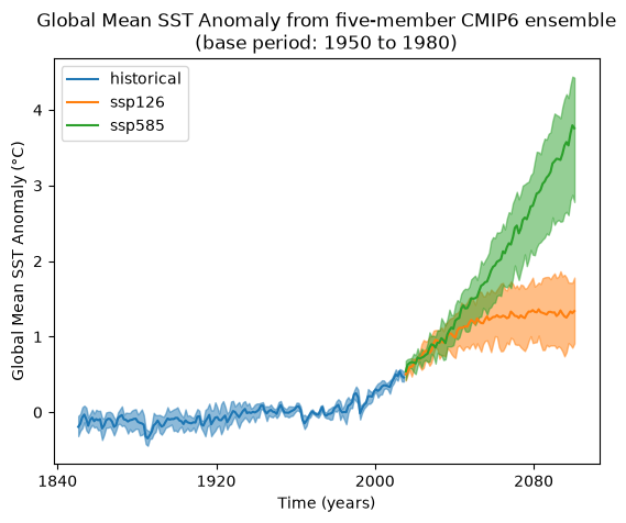
Let’s create a multi-model ensemble containing data from multiple CMIP6 models, which we can use to quantify our confidence in future projected sea surface temperature change under low- and high-emissions scenarios.

Your goal in this tutorial is to create a likely range of future projected conditions under both SSP 1-2.6 (low emissions) and SSP 5-8.5 (high emissions). The IPCC uncertainty language defines the likely range as the middle 66% of model results (ignoring the upper 17% and lower 17% of results)

Coding Exercise 2.1#

Complete the following code to display multi-model ensemble data with IPCC uncertainty bands:

Compute the multi-model mean temperature
Display the likely range of temperatures for the CMIP6 historical and projected data (include both SSP1-2.6 and SSP5-8.5) via shaded areas with da_upper and da_lower being the boundaries of these shaded regions.

#################################################
## TODO for students: Plot range of global mean SST anomaly for five-member ensemble##
# please remove the following line of code once you have completed the exercise:
raise NotImplementedError("Student exercise: Plot range of global mean SST anomaly for five-member ensemble")
#################################################

fig, ax = plt.subplots()
for experiment, color in zip(["historical", "ssp126", "ssp585"], ["C0", "C1", "C2"]):
    datasets = []
    for model in dt_gm_anomaly.keys():
        # calculate annual mean
        annual_sst = (
            dt_gm_anomaly[model][experiment]
            .ds.tos.coarsen(time=12)
            .mean()
            .assign_coords(source_id=model)
        )
        datasets.append(
            annual_sst.sel(time=slice(None, "2100")).load()
        )  # the french model has a long running member for ssp126
    # concatenate all along source_id dimension
    da = xr.concat(datasets, dim="source_id", join="override").squeeze()
    # compute ensemble mean and draw time series
    da.mean(...).plot(color=color, label=experiment, ax=ax)
    # extract time coordinates
    x = da.time.data
    # Calculate the lower bound of the likely range
    da_lower = da.squeeze().quantile(...)
    # Calculate the upper bound of the likely range
    da_upper = da.squeeze().quantile(...)
    # shade via quantile boundaries
    ax.fill_between(x, da_lower, da_upper, alpha=0.5, color=color)

# aesthetics
ax.set_title(
    "Global Mean SST Anomaly from five-member CMIP6 ensemble\n(base period: 1950 to 1980)"
)
ax.set_ylabel("Global Mean SST Anomaly (°C)")
ax.set_xlabel("Time (years)")
ax.legend()

# to_remove solution
fig, ax = plt.subplots()
for experiment, color in zip(["historical", "ssp126", "ssp585"], ["C0", "C1", "C2"]):
    datasets = []
    for model in dt_gm_anomaly.keys():
        # calculate annual mean
        annual_sst = (
            dt_gm_anomaly[model][experiment]
            .ds.tos.coarsen(time=12)
            .mean()
            .assign_coords(source_id=model)
        )
        datasets.append(
            annual_sst.sel(time=slice(None, "2100")).load()
        )  # the french model has a long running member for ssp126
    # concatenate all along source_id dimension
    da = xr.concat(datasets, dim="source_id", join="override").squeeze()
    # compute ensemble mean and draw time series
    da.mean("source_id").plot(color=color, label=experiment, ax=ax)
    # extract time coordinates
    x = da.time.data
    # Calculate the lower bound of the likely range
    da_lower = da.squeeze().quantile(0.17, dim="source_id")
    # Calculate the upper bound of the likely range
    da_upper = da.squeeze().quantile(0.83, dim="source_id")
    # shade via quantile boundaries
    ax.fill_between(x, da_lower, da_upper, alpha=0.5, color=color)

# aesthetics
ax.set_title(
    "Global Mean SST Anomaly from five-member CMIP6 ensemble\n(base period: 1950 to 1980)"
)
ax.set_ylabel("Global Mean SST Anomaly (°C)")
ax.set_xlabel("Time (years)")
ax.legend()

<matplotlib.legend.Legend at 0x7fa0508a5e90>

../../../_images/3add4c9069bb1bfb0ca24b0b2d08460b78083831986591f7052bd8c550a9c670.png

Submit your feedback#

Questions 2.1: Climate Connection#

What does this figure tell you about how the multi-model uncertainty compares to projected physical changes in the global mean SST?
Is this the same for both scenarios?
For a 5-model ensemble like this, how do the likely ranges specifically relate to the 5 individual model temperatures at a given time?

# to_remove explanation

"""
1. Under both of these scenarios (SSP1-2.6 and SSP5-8.5), the projected warming of the climate is greater than the multi-model uncertainty.
2. The warming is greater for SSP5-8.5, but so is the multi-model uncertainty, so the relative size of physical changes and multi-model uncertainty is comparable across both scenarios.
3. The likely range includes the middle 66% of model results at a given time. For 5 models this means the ranges encompass the middle 3 models (i.e., they exclude the highest and lowest valued model at each time).
"""

'\n1. Under both of these scenarios (SSP1-2.6 and SSP5-8.5), the projected warming of the climate is greater than the multi-model uncertainty.\n2. The warming is greater for SSP5-8.5, but so is the multi-model uncertainty, so the relative size of physical changes and multi-model uncertainty is comparable across both scenarios.\n3. The likely range includes the middle 66% of model results at a given time. For 5 models this means the ranges encompass the middle 3 models (i.e., they exclude the highest and lowest valued model at each time).\n'

Submit your feedback#

Summary#

In this tutorial, we have quantified the uncertainty of future climate projections by analyzing variability across a multi-model CMIP6 ensemble. We learned to apply the IPCC’s confidence levels to establish a likely range of projections, which refers to the middle 66% of model results, for multiple emission pathways.

Resources#

This tutorial uses data from the simulations conducted as part of the CMIP6 multi-model ensemble.

For a detailed explanation of the IPCC uncertainty language have a look at Box 1.1, Chapter 1 of the IPCC AR6, cf. p. 169-170.

For examples of how to access and analyze CMIP6 data, please visit the Pangeo Cloud CMIP6 Gallery.

For more information on what CMIP is and how to access the data, please see this page.

Tutorial 3: Quantifying Uncertainty in Projections

Contents

Tutorial 3: Quantifying Uncertainty in Projections#

Tutorial Objectives#

Setup#

Install and import feedback gadget#

Figure settings#

Helper functions#

Video 1: Quantifying Uncertainty in Projections#

Submit your feedback#

Submit your feedback#

Section 1: Loading CMIP6 Data from Various Models & Experiments#

Section 2: Quantifying Uncertainty in a CMIP6 Multi-model Ensemble#

Coding Exercise 2.1#

Submit your feedback#

Questions 2.1: Climate Connection#

Submit your feedback#

Summary#

Resources#